Custom autodiff part 1: the basics
If you’re working with an automatic differentiation system like PyTorch, JAX, or Flux.jl, a lot of the time you don’t have to think too much about how the magic happens. But every so often you might find yourself doing something that the framework doesn’t know how to differentiate properly. It’s also common that a custom autodiff “rule” will be more efficient when a function output is the result of an algorithm: matrix inversion, linear system solving, root-finding, etc.
The documentation for autodiff frameworks usually shows some way of implementing these kinds of custom “rules” (see for example the relevant pages for PyTorch, JAX, and Zygote.jl), but these pages typically don’t go into depth about how to derive them. And while there are some great resources for learning about how AD works in general, they usually stop short of explanations for what to do in these oddball cases. The goal of this series of posts is to write the tutorial I was looking for when I first ran into this.
I’m going to build on my last post, which walked through extending Andrej Karpathy’s micrograd to vector math, so I’ll illustrate simple implementations of some custom reverse-mode rules using my fork of micrograd. It might be helpful to look at that first, though I’ll try to make this series pretty self-contained.
One last note before we get started: my intent here is not to write a math treatise (nor am I really qualified to). Basically, I’m deliberately sacrificing some mathematical precision with the goal of writing an approachable tutorial for those of us whose eyes glaze over at phrases like “cotangent bundle”. If that troubles you, I’m guessing you may not really need a tutorial on this topic. That said, the documentation for ChainRulesCore.jl has a great writeup on this topic for anyone looking for a little more rigor (although they also caveat their own lack of rigor…), whether or not you’re actually using Julia. You could also read this first and then go check out their documentation.
Here’s what this series will cover:
- Part 1: Autodiff basics: forward- and reverse-mode
- Part 2: Linear maps and adjoints
- Part 3: Deriving forward-mode AD rules (w/ examples)
- Part 4: Deriving reverse-mode AD rules (w/ examples)
- Part 5: Putting it all together: differentiating constrained optimization
Let’s get to it!
Autodiff 101
We’ll start with the simple case of a function $y = f(x)$ that takes as input one vector $x \in \mathbb{R}^n$ and returns another $y \in \mathbb{R}^m$, which we can express as a map $f: \mathbb{R}^n \rightarrow \mathbb{R}^m$. This actually won’t really cover a lot of practical cases, but hopefully it’ll be a good way to get a feel for the basic mechanics. In later parts we’ll see how to extend the basic version to more general cases.
The purpose of automatic differentiation (AD) is computing the derivative of the result of some numerical computation with respect to the inputs. AD systems assume that even highly complex functions can be decomposed into a sequence (or graph) of relatively simple primitive operations, each of which can be analytically differentiated in isolation. Under that assumption, the derivative of complex functions can be decomposed into a second graph of the derivatives of the primitive operations using the chain rule from calculus.
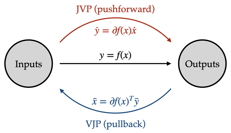
The way that the analytic derivatives are implemented is in terms of rules for Jacobian-vector products (in forward mode) and vector-tranpose-Jacobian products (in reverse mode). So for $f: \mathbb{R}^n \rightarrow \mathbb{R}^m$, we can think of its derivative at some nominal input values $x \in \mathbb{R}^n$ is the Jacobian matrix $\partial f(x) \equiv df/dx \in \mathbb{R}^{m \times n}$. The Jacobian-vector product (JVP) applied to a “tangent” vector $v \in \mathbb{R}^n$ essentially implements the matrix-vector multiplication
\[\partial f(x) v.\]Why is this useful? The key thing is that JVP rule can usually evaluate this product without explicitly constructing the Jacobian.
If the input is scalar-valued, then $v \in \mathbb{R}$ and this JVP with $v = 1$ will return the derivative of $f$ at $x$, giving the sensitivity of the outputs to the inputs near the nominal input $x$. On the other hand, if the input is vector-valued, reconstructing the full Jacobian would require evaluating the JVP $n$ times, for instance using the unit basis vectors as tangent vectors $v$. When $n$ is large this becomes very expensive, but fortunately it is rarely necessary to explicitly form the full Jacobian; many algorithms boil down to a series of linear system solves, and iterative linear solvers like CG and GMRES only really need to evaluate the matrix-vector product, which is exactly what the JVP provides.
As we’ll see, the Jacobian-vector product (also known as the pushforward) is the building block of forward-mode autodiff. Similarly, the vector-Jacobian product (also known as the pullback) is the main building block of reverse-mode autodiff. For the same function $f: \mathbb{R}^n \rightarrow \mathbb{R}^m$ above, the vector-Jacobian product (VJP) applied to an “adjoint” (or “covariant”, or “dual”) vector $w \in \mathbb{R}^m$ implements the vector-transpose-matrix multiplication
\[w^T \partial f(x_0).\]This can also be viewed as a matrix-vector multiplication with the transpose or adjoint of the Jacobian $\partial f(x)^T \in \mathbb{R}^{n \times m}$:
\[\partial f(x)^T w.\]Note that while the seed of the Jacobian-vector product is an element of the input space, the seed for the vector-Jacobian product is an element of the output space (technically this is not quite true, but it’s close enough for our purposes). In a sense, these “adjoint” vectors represent perturbations of the function outputs, and reverse-mode autodiff is responsible for computing corresponding perturbations of the function inputs.
This might be a little counterintuitive: we need Jacobians for a lot of different numerical methods and sensitivity analyses in scientific computing, so it might make sense that an efficient Jacobian-vector product would be useful, but when do we ever need the transpose of the Jacobian? Much less, what good is the product of the transpose with some particular vector? There’s one context in particular that’s very important and where it turns out that the vector-Jacobian product is exactly what we need: optimization.
Let’s say we have an unconstrained optimization problem with decision variables (parameters) $\theta \in \mathbb{R}^n$. The optimization problem for a scalar-valued cost function $J(\theta)$ is
\[\min_\theta J(\theta).\]In order to solve this problem, a key piece of information is the gradient of $J$ evaluated at some particular set of parameters $\theta$. Since the cost function maps from $\mathbb{R}^n$ to $\mathbb{R}$, we usually think of the gradient as a vector $\nabla J(\theta) \in \mathbb{R}^n$.
How do we get this gradient using automatic differentiation? The Jacobian for a function $f: \mathbb{R}^n \rightarrow \mathbb{R}$ is a matrix (basically a row vector) $\partial J(\theta) \in \mathbb{R}^{1 \times n}$. Hence, the gradient is effectively the transpose of the Jacobian: $\nabla J(\theta) = \partial J(\theta)^T$.
In forward-mode autodiff what we get is the Jacobian-vector product with some seed vector $v \in \mathbb{R}^n$, which amounts to a dot product with the gradient: $\partial J(\theta) v = \nabla J(\theta) \cdot v$. So in order to evaluate the full gradient using forward-mode autodiff, we would need to compute $n$ Jacobian-vector products, using as seed vector each of the $n$ standard basis vectors like $e_1 = \begin{bmatrix} 1 & 0 & 0 & \cdots \end{bmatrix}^T$.
On the other hand, in reverse-mode autodiff what we get is the vector-Jacobian product with a seed value $w \in \mathbb{R}$, which is essentially a rescaled gradient: $\partial J(\theta)^T w = w\nabla J(\theta)$. If we happen to choose $w=1.0$ as the seed value, then we immediately get the gradient $\nabla J(\theta)$ using only a single vector-Jacobian product.
This is what makes reverse-mode AD (a.k.a. backpropagation) so powerful in the context of optimization. It only requires a single backwards pass with about the same computational complexity as the forwards pass to compute the full gradient, no matter how many input variables there are. For the same reason, reverse-mode AD is much more efficient at computing full Jacobians for functions with many more inputs than outputs; again, you just have to do a VJP seeded with a standard basis vector for each row of the Jacobian. There’s a very naive (but hopefully easy to follow) implementation of this in micrograd.functional.
Static vs dynamic data
We’ll often write and/or implement functions using a number of variables, not all of which are really “inputs”. For example, if we write a function $f(x) = ax$, then the variable $a$ is neither an input not an output to the function. In a sense it just parameterizes the function.
Variables like this are sometimes called “static” data, as opposed to “dynamic” data that can change depending on the inputs. We don’t have to account for these in our derivations of the autodiff rules, and we should be careful to implement the functions in such a way that it is clear what data is static and what is dynamic. However, you always can make them dynamic by treating them as additional arguments to the function and deriving autodiff rules for them as well. In general it might be helpful to treat as many variables as possible as dynamic – you never know what you might want to optimize.
For instance, if we have function representing a matrix-vector product $f(x) = A x$, then the matrix $A$ is static data and the Jacobian is $\partial_x f = A$. On the other hand, if we wrote the function as $f(A, x) = A x$, then both $A$ and $x$ are dynamic and the Jacobian has two parts: $\partial_x f = A$ and $\partial_A f = x$. The derivative with respect to $x$ is obviously unchanged, but now we also have to account for variations in $A$.
This may seem obvious but sometimes it can be a bit tricky to keep track of, particularly in machine learning applications. For example, suppose we have a neural network $f_\theta(x)$, where $\theta$ are the various weights and biases in the network. In the context of training this network the inputs to a neural network are samples $x$ from the training data, and the outputs are the predictions $y = f_\theta(x)$…. right?
But really, the training task is to minimize some loss function over a training set ${ (x_i, y_i) }_{i=1}^N$:
\[\min_\theta \frac{1}{N} \sum_{i=1}^N \mathcal{L}(\hat{y}_i, y_i), \qquad \hat{y}_i = f_\theta(x_i).\]From this point of view the function we actually want to differentiate is
\[J(\theta) = \frac{1}{N} \sum_{i=1}^N \mathcal{L}(f_\theta(x_i), y_i).\]The real inputs are the weights and biases $\theta$! The training data are not inputs, but static data. That is, we don’t need to calculate the derivative of anything with respect to the data itself in the training process. That’s not to say you never need the Jacobian $\partial_x f$ for anything, but you don’t need it for training; all you need is the Jacobian $\partial_\theta f$.
This can be hard to keep track of, especially since $\theta$ are often called parameters and $x$ and $y$ are inputs and outputs. Just try to think carefully about what you actually need to compute the sensitivity of, and with respect to what inputs.
Composing functions
If $f$ represents a complex calculation – like a partial differential equation solve or prediction from a machine learning model – it becomes more and more difficult to compute the linearization $\partial f (x)$ analytically. The key insight of AD systems is that often $f$ is composed of a large number of simpler functions, in which case the chain rule says that the Jacobian is a series of matrix-vector products.
For instance, if $f(x) = g(h(x))$, where we know how to calculate the Jacobian-vector product (pushforward) for both $g$ and $h$, then
\[\partial f(x) v = \partial g(h(x)) \partial h(x) v.\]Note that the nominal inputs to $g$ are the outputs from $h$ at its nominal inputs $x$, and the tangent vector for the JVP for $g$ is the output of the JVP for $h$. We can calculate the full JVP by propagating both the nominal (or “primal”) and tangent values through the computational graph in parallel:
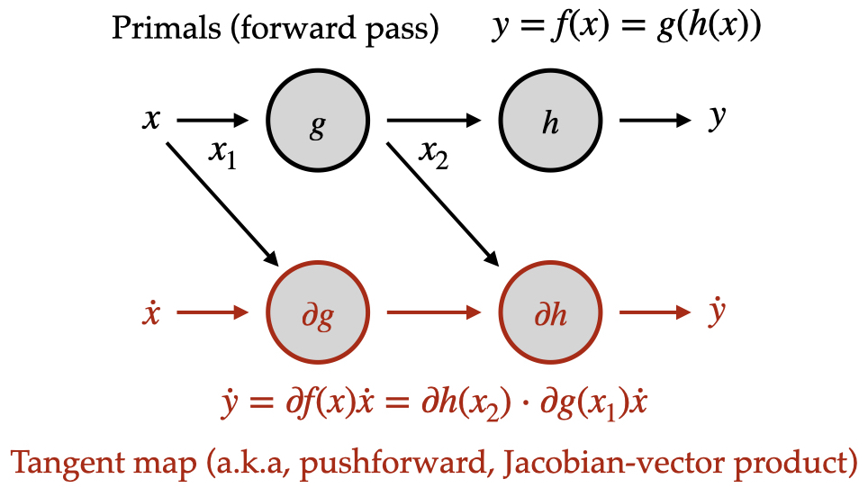
- Begin with the nominal input value $x_1$ and seed vector $\dot{x}_1$.
- Compute the nominal output $x_2 = g(x_1)$ and pushforward $\dot{x}_2 = \partial g(x_1) \dot{x}_1$.
- Compute the nominal output $y = h(x_2)$ and pushforward $\dot{y} = \partial h(x_2) \dot{x}_2$.
- Finally, the nominal output is $y$ and the result of the JVP is $\dot{y}$.
All information required to compute each component Jacobian-vector product is passed via the primal and tangent vectors. This means that the forward-mode rule for some primitive function can be implemented in complete isolation. Basically, your function will be somewhere in this chain.
As the implementer of the pushforward (Jacobian-vector product), you can expect to be handed a seed vector (an element of the input space) along with the nominal input values and your job is to calculate the pushforward (returning an element of the output space).
Here’s a simple example borrowed from the JAX documentation implementing the pushforward (JVP) for the function $f(x, y) = y \sin(x) $.
Since this is basically a scalar function (you don’t have to worry too much about broadcasting, ufuncs, etc in JAX), it’s easy to calculate the derivatives with basic calculus.
Note that the JVP is basically the total derivative: if $z = f(x, y)$, the value tangent_out is $\dot{z}$, where
We’ll explain that and build on it further later, for now just take a quick look at the code to get a feel for the structure – maybe you can recognize some of the pieces we’ve already talked about.
import jax.numpy as jnp
from jax import custom_jvp

@custom_jvp
def f(x, y):
  return jnp.sin(x) * y

@f.defjvp
def f_jvp(primals, tangents):
  x, y = primals
  x_dot, y_dot = tangents
  primal_out = f(x, y)
  tangent_out = jnp.cos(x) * x_dot * y + jnp.sin(x) * y_dot
  return primal_out, tangent_out
In a sense, the vector-Jacobian product (pullback) just performs the products in the chain rule in the opposite order. The pullback for $f(x) = g(h(x))$ expands to
\[w^T \partial f(x) = w^T \partial g(h(x)) \partial h(x).\]Calculating this presents a bit of a puzzle. The vector-transpose-matrix products propagate from left to right, but $g$ still requires as its inputs the nominal outputs $h(x)$, implying that the primal calculation has to be completed before the VJP. This is the root of the “forward/backwards” passes in the reverse-mode algorithm. The primal calculation is fully completed first, with all intermediate values stored. Then the pullback can be calculated by propagating the adjoint values backwards through the computational graph:
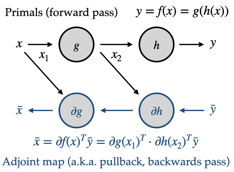
- Begin with the nominal input value $x$ and seed vector $\bar{y}$.
- Compute the intermediate primal output $x_2 = g(x_1)$. Save this value for later.
- Compute the final primal output $y = h(x_2)$.
- Compute the VJP for the second function: $\bar{x}_2 = \partial h(x_2)^T \bar{y}$.
- Compute the VJP for the first function: $\bar{x}_1 = \partial g(x)^T \bar{x}_2 \equiv \bar{x}$.
- The full VJP $\partial f(x)^T \bar{y}$ is $\bar{x}$.
Note that the full “forward pass” happens first, storing intermediate results, and then the “backwards pass” happens, using stored primal values from the forward pass.
Again, your custom function will happen somewhere in this process. As the implementer of the pullback (vector-Jacobian product), you will implement one stage of the backwards pass: you can expect to be handed an adjoint vector (an element of the output space) along with the nominal input/output values and your job is to calculate the pullback (returning an element of the input space).
Here’s the same example as before borrowed from the JAX docs, but this time implementing the VJP.
As before, it’s easy enough to calculate these derivatives by hand.
This time note that what gets returned is the gradient of the output evaluated at the nominal values, scaled by the adjoint value w.
For a scalar function (or ufunc in this case), that’s the same thing as the vector-Jacobian product (but here the “vector” is just the scalar w).
from jax import custom_vjp

@custom_vjp
def f(x, y):
  return jnp.sin(x) * y

def f_fwd(x, y):
# Returns primal output and residuals to be used in backward pass by f_bwd.
  return f(x, y), (jnp.cos(x), jnp.sin(x), y)

def f_bwd(res, w):
  cos_x, sin_x, y = res # Gets residuals computed in f_fwd
  return (cos_x * w * y, sin_x * w)

f.defvjp(f_fwd, f_bwd)
Looking ahead
In this post we covered some of the basic concepts of automatic differentiation applied to functions with vector inputs and outputs. This is laying some groundwork for Part 2, where we’ll see how to generalize the Jacobian, JVP, and VJP to functions that operate on all kinds of different inputs. That part will be a little math-heavy, but then we will be able to fully understand the process of deriving custom autodiff rules.