Differentiating through differential equations
In my last series of posts, I tried to lay out a basic approach to deriving “custom autodiff rules”; essentially, computing the parametric sensitivity of a function for use in either forward- or reverse-mode automatic differentiation frameworks.
That’s all well and good for basic math operations, but it can be tricky to apply that kind of procedure to more complex computations. Specifically, this becomes important in scientific computing, where the “function” represents a numerical discretization of some continuous model of the physical world in the form of a differential equation (ordinary, partial, stochastic, whatever). In these domains efficiently evaluating sensitivities to a large number of parameters can be critical for optimal control, design optimization, system identification, surrogate modeling, data assimilation, and related applications.
It is possible to just implement your entire differential equation solver in some automatic differentiation framework (for instance torchdiffeq, diffrax, or many of the Julia solvers). However, that assumes you’re willing to do the work of implementing your solver more or less from scratch in one of these frameworks, unless it happens to be something that is supported already. Besides which, these frameworks tend to be optimized for machine learning and not scientific computing, so even if you’re trying to do some “scientific machine learning” application, you still might want to outsource your actual scientific computing to some other library (Julia is an exception here, although in my opinion their PDE-solving capabilities lag far behind their ODE/DAE/SDE solvers).
All that to say, in these cases it can be worthwhile to go back to the drawing board and derive the sensitivity equations from scratch. In this post, I’ll try to give a quick rundown of my preferred approach: Lagrange multipliers and the continuous adjoint method. I would also recommend two other sources on this: a short tutorial by Andrew Bradley on adjoint methods and the writup on the mathematical background of adjoints by Patrick Farrell on the pyadjoint documentation website.
ODE-constrained optimization
Let’s take the following optimization problem:
\[\begin{gather} \min_p J(x(t_f)) \\ \dot{x} = f(x, p), \qquad x(0) = x_0. \end{gather}\]Here $x(t)$ is the time-varying state vector whose evolution is governed by the (autonomous) ODE $\dot{x} = f(x, p)$, and $p$ is some vector of parameters or decision variables. This is a common problem structure in optimal control, for instance, where the cost $J(x(t_f))$ might penalize the difference between the state of the system and some commanded state, and $p$ might be spline coefficients that determine the inputs to the system as a function of time. This might also represent a parameter estimation problem, where $J$ is the deviation between some measurement of the system and the simulated predictions, and $p$ are the physical parameters of the model that we would like to calibrate.
This form can also be generalized in a number of ways; the cost function could also depend directly on the parameters, the initial or final state could also be functions of the variables, the ODE could have time dependence, the ODE could be a differential-algebraic equation (DAE) or partial differential equation (PDE), and so on. We’ll come back to this at the end
The question is, how do we compute the gradient of $J$ with respect to $p$ subject to the constraint that $x(t)$ must satisfy the ODE? In the earlier posts, we basically relied on the chain rule and implicit function theorem. That is, view $x$ as a function of $p$ and so $J = J(x(p))$ and
\[\frac{dJ}{dp} = \frac{dJ}{dx}\frac{dx}{dp},\]and then we just have to compute each of the two terms. But what does $dx/dp$ mean when $x$ represents a continuous trajectory and not a fixed value?
Another way to look at the same problem is to wade into the calculus of variations. Since $\dot{x} - f(x, p) = 0$, we can add any multiple of this quantity to the cost function without changing its value:
\[J(x(t_f)) = J(x(t_f)) + \int_0^{t_f} \lambda^T \left( \dot{x} - f(x, p) \right) ~ dt \equiv L(x, p, \lambda).\]$L$ here is the Lagrangian, and we’ve introduced the Lagrange multipliers $\lambda(t)$, a time-varying vector which has the same dimensions as $x(t)$ and is often called the “adjoint state”, for reasons that will become clear. The important thing is that since $\dot{x} - f(x, p) = 0$, we can choose $\lambda(t)$ to have any values we want; in the next section we will find a specific choice of $\lambda$ that lets us efficiently compute the derivative of the cost function.
From the Lagrangian to the adjoint
Provided that $x(t)$ is a solution to the ODE, $L$ and $J$ are equal, and so $dJ/dp = dL/dp$. On the surface, it’s not clear we’ve gained anything yet by introducing the Lagrangian and the Lagrange multipliers. However, expanding the derivative of the Lagrangian, we at least have more to work with now:
\[\frac{dL}{dp} = \left. \frac{dJ}{dx}\frac{dx}{dp} \right|_{t=t_f} + \int_0^{t_f} \left[\frac{d \lambda^T}{dp} \left( \dot{x} - f(x, p) \right) + \lambda^T \left( \frac{d \dot{x}}{dp} - \frac{\partial f}{\partial x}\frac{dx}{dp} - \frac{\partial f}{\partial p} \right) \right] ~ dt.\]This still doesn’t look helpful. We still have this mystery term $dx/dp$ all over the place, and even its time derivative $d\dot{x}/dp$. However, we can make a couple of crucial simplifications, and ultimately the goal will be to define the function $\lambda(t)$ such that we never have to actually directly compute $dx/dp$.
First, since $\dot{x} = f(x, p)$, we can eliminate the term with $\frac{d \lambda^T}{dp}$ altogether. Second, we can integrate $\lambda^T \frac{d\dot{x}}{dp} $ by parts:
\[\begin{align} \int_0^{t_f} \lambda^T \frac{d\dot{x}}{dp} ~ dt &= \int_0^{t_f} \lambda^T \frac{d}{dt}\frac{dx}{dp} ~ dt \\ &= \left[ \lambda^T \frac{dx}{dp} \right]_0^{t_f} - \int_0^{t_f} \dot{\lambda}^T \frac{dx}{dp} ~ dt. \end{align}\]The first term contains the boundary values from integration by parts; fortunately, since the initial condition $x(0)$ has no dependence on $p$, we know that
\[\left. \frac{dx}{dp} \right|_{t=0} = 0.\]As for the boundary value at $t=t_f$, evaluating it directly would require knowing $dx/dp$ at the final time. Let’s leave the boundary term from the final time for now, so that the integration by parts is
\[\int_0^{t_f} \lambda^T \frac{d\dot{x}}{dp} ~ dt = \left. \lambda^T \frac{dx}{dp} \right|_{t=t_f} - \int_0^{t_f} \dot{\lambda}^T \frac{dx}{dp} ~ dt.\]Let’s return to the derivative of the Lagrangian with these changes, and rewrite the integrand to group terms that multiply $dx/dp$:
\[\frac{dL}{dp} = \left. \left( \frac{dJ}{dx} + \lambda^T \right) \frac{dx}{dp} \right|_{t=t_f} - \int_0^{t_f} \left\{ \left[\dot{\lambda}^T + \lambda^T \frac{\partial f}{\partial x} \right] \frac{dx}{dp} + \lambda^T \frac{\partial f}{\partial p} \right\} ~ dt.\]Let’s start with the first set of terms (those evaluated at $t=t_f$). So far we have not imposed any requirements on $\lambda(t)$, but we know that we can define it however is convenient. In this case, it would be convenient if the term in parentheses was zero, so that we did not have to compute $\frac{dx}{dp}$ at $t_f$. This means that we should choose
\[\lambda(t_f) = -\left( \frac{dJ}{dx} \right)^T_{t=t_f} \equiv -J'(x(t_f))^T.\]Then our equation for the gradient of the Lagrangian simplifies to
\[\frac{dL}{dp} = - \int_0^{t_f} \left\{ \left[\dot{\lambda}^T + \lambda^T \frac{\partial f}{\partial x} \right] \frac{dx}{dp} + \lambda^T \frac{\partial f}{\partial p} \right\} ~ dt.\]Finally, we’ll make one last leap: we have chosen a value for $\lambda(t)$ at $t_f$, but not at any other time. If we really don’t want to compute $dx/dp$ (or even worry too much about how we would compute it), the easiest thing to do is to use that flexibility to require that the term in square brackets is also zero:
\[\dot{\lambda}^T + \lambda^T \frac{\partial f}{\partial x} = 0,\]or, taking the transpose of this and isolating $\dot{\lambda}$,
\[\dot{\lambda} = - \left(\frac{\partial f}{\partial x}\right)^T \lambda.\]Essentially, we’ve defined a new ODE that governs the evolution of $\lambda(t)$. Together with the condition that $\lambda(t_f) = 0$, we can interpret this as a “terminal-value problem”, or an ODE that runs backwards in time from $t_f$ to $t=0$ starting from $\lambda(t_f) = 0$. We can also see why this is called the “adjoint” method: $\partial f/\partial x$ is the Jacobian of $f$, and the evolution equation for $\lambda$ is a linear ODE using the transpose of that Jacobian, or the adjoint linear operator. For instance, if the original ODE was linear ($\dot{x} = A(p) x$), then $(\partial f/\partial x)^T = A(p)^T$.
Importantly, unless the system is linear and time-invariant this is a time-varying Jacobian; as the adjoint system evolves backwards in time, the linearization of the ODE system must be done about the forward solution $x(t)$. This introduces some practical challenges, but let’s set that aside for now.
The final form of the gradient of the Lagrangian is then
\[\frac{dL}{dp} = - \int_0^{t_f} \lambda^T \frac{\partial f}{\partial p} ~ dt.\]The optimization procedure
Putting this all together, we can compute the gradient of $J$ with respect to $p$ as follows:
- Solve the original ODE forward in time from $t=0$ to $t_f$:
-
Given the solution $x_f = x(t_f)$, compute the cost function $J(x_f)$ and its derivative $J’(x_f)$
-
Solve the adjoint system backwards in time from $t_f$ to $t=0$:
- With both the forward and adjoint solutions computed, calculate the gradient via quadrature:
As with the other reverse-mode autodiff or “backprop” methods, this method does not depend on the number of parameters, except for the final quadrature step! It always requires only one forward solve and one adjoint solve to compute the gradient of $J$ with respect to any number of parameters. This has made it a method of choice for fields like neural ODEs, where the dimension of $p$ might be quite large.
Practical considerations
Once you wrap your head around the tricks involved in adjoint-based optimization, the procedure outlined above can seem simple enough: solve the original ODE forward in time, solve the adjoint ODE backward in time, and then compute the gradients. However, there are two main difficulties in putting this into practice.
Interpolation and checkpointing
The first issue is computing the various derivatives like $\partial f/\partial x$, and $\partial f/\partial p$. Remember that these must be evaluated as the linearizations of $f(x, p)$ about the current values of the forward solution $x(t)$. However, most practical ODE solvers are adaptive time-stepping algorithms, so in all likelihood we won’t really know exactly what $x(t_k)$ is for any particular step $t_k$ in the adjoint solve.
One approach is the “backsolve”: solving the original ODE backwards in time at the same time as the adjoint. We know the final value of the original ODE as a result of the forward solve (call it $x_f$), so we could just integrate backwards in time alongside the adjoint equation:
\[\begin{align} \dot{x} &= f(x, p), \qquad x(t_f) = x_f \\ \dot{\lambda} &= - \left(\frac{\partial f}{\partial x}\right)^T \lambda, \qquad \lambda(t_f) = 0. \end{align}\]From an efficiency point of view this isn’t ideal, since the state vector is doubled and the ODE solve becomes more expensive accordingly. Still, it’s one of the more common solutions to this problem (also recently popularized by the neural ODEs paper, but I believe was widely used in the optimal control community as part of “direct single shooting” schemes long before that).
Another approach to interpolation is to use the interpolant associated with the forward solution (usually computed as part of the “dense output” of most ODE solvers) to approximate $x(t_k)$. I have had issues with accuracy in this approach (but possibly more related to numerical stability), but typically the main drawback to this is when the system size is large, since all the information needed to reconstruct the solution interpolant must be stored in memory. This is usually addressed with “checkpointing”, which tries to balance computational cost and memory cost by storing the solution at intermediate times and re-doing the forward solve as necessary between the checkpoints (see for instance the description in the CVODES docs).
Numerical stability
The second issue is numerical stability. I don’t know of specific conditions for this, but reportedly the “backsolve” method is often numerically unstable. In my experience, it often seems to be okay for relatively short time horizons and becomes unstable over long times. To some extent, tighter tolerances can help, but only up to a point.
We can see this with a simple scalar ODE:
\[\dot{x} = -ax, \qquad x(0) = x_0.\]For $a > 0$, the system is linearly stable and the solution is a damped exponential: $x(t) = x_0 e^{-at}$. The adjoint system is:
\[\dot{\lambda} = a\lambda , \qquad \lambda(t_f) = 0.\]This ODE is linearly unstable forward in time, but since we’re solving it backwards in time, we effectively flip the sign of the right-hand side, so this is also okay. Specifically, would usually accomplish the backwards solve by defining $\tau = -t$ and solving the initial value problem from $\tau = -t_f$ to $\tau = 0$
\[\frac{d \lambda}{d \tau} = - \frac{d \lambda}{dt} = -a\lambda, \qquad \lambda(-t_f) = 0.\]Again, this is a stable system, so numerically it shouldn’t pose any problems. The trouble comes in when we try to augment the system with the backwards solution of the original ODE. Now the “negative time” ODE system is
\[\begin{align} \frac{dx}{d\tau} &= a x, \qquad x(-t_f) = x_0 e^{-a t_f}, \\ \frac{d \lambda}{d \tau} &= -a\lambda, \qquad \lambda(-t_f) = 0. \end{align}\]Now the original ODE becomes unstable when run backwards in time! On paper this is still okay, since we will just run the solution back to $x_0$, but in practice small numerical errors also grow like $e^{a\tau}$ and can become significant over longer integration horizons.
For instance, here’s what happens if we solve this system with $a=1$ over $t_f = 10$: so far no problems (SciPy Dormand-Prince solver with rtol=1e-3 and atol=1e-6):
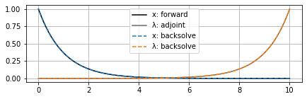
However, if we extend the time horizon out a little farther, now we can see the backsolve for $x$ (again, remember this starts from the right at $t_f$ and moves left to $t=0$) start to blow up, even though $\lambda$ is still okay:
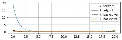
This can also be overcome by a checkpointing-type method where the state $x$ is reset to its forward values at certain points. Then even if numerical errors start to accumulate, hopefully they don’t grow to the point where they interfere significantly with the gradient estimate before the next checkpoint is reached and $x$ is reset to its correct value.
The folks at Julia Computing put out an interesting paper a few years ago with a fairly extensive analysis of different adjoint methods, where they discuss both stability considerations and interpolation/checkpointing.
As a final comment on stability, note that if we had $\dot{x} = ax$ so that the original ODE was unstable, then the adjoint ODE would be $\dot{\lambda} = -a\lambda$, which is stable forward in time but also unstable backwards in time. In this case the stability problem is more fundamental and doesn’t have anything to do with the implementation of the adjoint solve; it’s just reflecting that the solution becomes exponentially more sensitive over time. Chaotic systems have a similar effect as a result of their sensitivity to initial conditions.
Micrograd implementation
As in the custom autodiff series, I think it is helpful to see a basic implementation of the method to understand it. Again, I’ll use my fork of Andrej Karpathy’s micrograd engine to demonstrate, and we’ll use SciPy for the ODE solver. This fork has some modifications (described in this post) to work with arrays and support vector-Jacobian products and a JAX-inspired functional interface. The implementation of the backwards pass for the ODE solve is more complex than the examples in that first post, but generally follow the pattern from the series on custom autodiff rules.
To have a really minimal version of this, I’ll make the following simplifications
- Use the dense interpolant from the forward solve as the primal values for linearization in the backwards pass
- Support only the “RK45” (Dormand-Prince) method from SciPy
- Only allow differentiation with respect to a vector of parameters (not the initial condition or the boundary times)
- Return only the final value of the ODE solve and not any intermediate time series
That is, the input function must have the signature fun(t, y, p) -> dy/dt, where t is the independent variable, y is the state of the system, and p are the parameters of the system.
The function should be written to accept and return micrograd.Array objects (constructed similar to NumPy with micrograd.array(x)).
Here’s the full code for odeint, and then I’ll break it down piece by piece:
import numpy as np
from scipy.integrate import solve_ivp, quad_vec

from micrograd.engine import Array


def odeint(fun, t_span, y0: np.ndarray | Array, p: Array, rtol=1e-3, atol=1e-6):
    """Integrate a system of ordinary differential equations."""

    if isinstance(y0, Array):
        y0 = y0.data

    solver_options = {
        "method": "RK45",
        "rtol": rtol,
        "atol": atol,
        "args": (p.data,),
        "dense_output": True,
    }

    # The function should be written to accept and return micrograd.Array objects,
    # but the SciPy solver will pass in and expect NumPy arrays, so we need to
    # wrap the user function to convert between the two.
    def ode(t, y, p):
        y_mg, p_mg = Array(y), Array(p)
        return fun(t, y_mg, p_mg).data

    # Forward pass: call SciPy to compute the solution
    # Use the dense_output=True option to get a callable solution that can be
    # used for computing Jacobians during the backwards pass
    fwd = solve_ivp(ode, t_span, y0, **solver_options)
    x = fwd.sol  # Interpolant that can be called with x(t)

    # Return value as a micrograd.Array.  The `_backward` method will be
    # defined via the adjoint solve below.
    out = Array(fwd.y[:, -1], (p,), 'odeint')

    # Evaluate the VJP (df/dx)^T * v and (df/dp)^T * v at time t
    # Accepts numpy arrays as inputs for `t`, `v`, and `p`.
    # This avoids directly computing the Jacobian by using
    # reverse-mode autodiff applied to the dynamics function
    # to compute both VJPs simultaneously with no additional cost.
    def f_vjp(t, v, p, var='x'):
        y, p = Array(x(t)), Array(p)
        dy = fun(t, y, p)
        dy.backward(gradient=v)
        return y.grad, p.grad

    # Adjoint dynamics: -(df/dx)^T * lambda
    def f_adj(t, lambda_, p):
        return f_vjp(t, lambda_, p)[0]  # First output is df/dx

    def _backward():
        # The seed vector will be in `out.grad`; this will initialize the
        # adjoint state at t=tf.
        lambda_ = out.grad
        adj = solve_ivp(f_adj, t_span[::-1], lambda_, **solver_options)

        def _quad(t):
            # Compute (df/dp)^T * lambda
            return -f_vjp(t, adj.sol(t), p.data)[1]  # Second output is df/dp

        # Compute the integral of the adjoint state for every parameter
        dJ, _err = quad_vec(_quad, *t_span)
        p.grad += dJ

    out._backward = _backward
    return out
The first part of the function is fairly self-explanatory; this is just conversions back and forth between NumPy and micrograd array types.
The input fun should work with micrograd arrays so that we can differentiate it with our autodiff system, but SciPy will pass and expect NumPy arrays.
The real work starts with the forward pass, where we call scipy.integrate.solve_ivp to generate the “primal” solution.
Note that the solver options include a request for the “dense output”, which will provide an interpolant we can call with x(t) for any value of t in the tspan to get an approximation of the primal solution at that time.
As discussed above, this is not a particularly efficient way to do this, but it’s simple and relatively stable.
We’ll hold onto this solution for use in the backwards pass (defining the _backward function in the same function scope will keep the forward solution in Python’s memory for as long as it’s needed).
The next important component is the f_vjp function:
def f_vjp(t, v, p, var='x'):
    y, p = Array(x(t)), Array(p)
    dy = fun(t, y, p)
    dy.backward(gradient=v)
    return y.grad, p.grad
It might not look much like it, but this is essentially the right-hand side of the adjoint ODE
\[\dot{\lambda} = \left(\frac{\partial f}{\partial x}\right)^T \lambda\]As discussed in the “beefing up micrograd” post, when the backward method of a micrograd array y = f(x) is “seeded” with the argument gradient=v, what actually gets computed is the vector-Jacobian product (or, really, the Jacobian-transpose vector product) $(\partial f/\partial x)^T v$.
When y is a scalar, by default v=1 and this is equivalent to computing the gradient with respect to x.
So when we call f_vjp with $\lambda$ as the value for v and then evaluate dy.backward(gradient=v), what we compute is
just as required for the adjoint ODE.
The value about which we linearize is x(t), the interpolated value of the primal solution from the forward ODE solve.
As a bonus, the backwards pass will also compute the vector-Jacobian product for the Jacobian with respect to the parameters, so we get
basically “for free”.
We don’t need that to solve the adjoint ODE, but we do need it to compute the final gradient, so f_vjp is written to return both, and then f_adj just grabs the first of these values to use in the adjoint ODE solve.
The next part of the code is the actual backwards pass associated with the odeint function:
def _backward():
    # The seed vector will be in `out.grad`; this will initialize the adjoint state at t=tf.
    lambda_ = out.grad
    adj = solve_ivp(f_adj, t_span[::-1], lambda_, **solver_options)

    def _quad(t):
        # Compute (df/dp)^T * lambda
        return -f_vjp(t, adj.sol(t), p.data)[1]  # Second output is df/dp

    # Compute the integral of the adjoint state for every parameter
    dJ, _err = quad_vec(_quad, *t_span)
    p.grad += dJ
The first part of this solves the adjoint ODE terminal-value problem starting with the value “seeded” from any upstream backwards pass computations in the output array, which becomes the value of $\lambda$ at $t_f$. Again, the SciPy solver is asked to return the dense interpolant as part of the adjoint solution.
Now we have everything we need to compute the actual gradient
\[\frac{dJ}{dp} = -\int_{t_0}^{t_f} \lambda^T \frac{\partial f}{\partial p} ~ dt.\]This integral can be computed efficiently via numerical quadrature, implemented in SciPy in the quad_vec function.
As with the adjoint ODE, the integrand is really just a vector-Jacobian product where the vector is $\lambda$ and the Jacobian is now with respect to the parameters and not the state.
Hence, we can evaluate the integrand efficiently using f_vjp, this time returning the second value to get $(\partial f/\partial p)^T \lambda$.
This happens in the _quad function.
Finally, we just accumulate this integral to the .grad array for the parameters.
As a simple example, the following code computes the parameteric sensitivity of the ODE for a point mass subject to gravity and quadratic drag:
\[\ddot{y} = -\frac{b}{m} \dot{y}^2 - g\]import numpy as np
import micrograd as mg
def f(t, y, p):
x, v = y[0], y[1]
b, m, g = p
return mg.array([v, -b/m*v**2 - g])
t_span = (0, 1)
y0 = np.array([0.0, 10.0])
p = mg.array([0.0, 1.0, 9.8])
y = mg.odeint(f, t_span, y0, p)
# Seed the gradient with [1, 0], taking the sensitivity of the
# final height with respect to the parameters (b, m, g)
y.backward(gradient=np.array([1.0, 0.0]))
print(p.grad) # dy(tf)/dp = [-25.33666667, 0. , -0.5 ]
Generalizing the problem
Now that we’ve seen the basics of deriving adjoint methods with the Lagrangian approach, let’s wrap up by revisiting the original optimization problem to see a few ways it can be generalized. I won’t go through the derivations of these, but all of them can be done with the same basic approach (albeit sometimes with a few extra pieces of paper).
The original optimization problem was written as
\[\begin{gather} \min_p J(x(t_f)) \\ \dot{x} = f(x, p), \qquad x(0) = x_0. \end{gather}\]The first way we could generalize this is to allow parametric dependence in the cost function and support a “running cost” term:
\[\begin{gather} \min_p J_f(t_f, x(t_f), p) + \int_{t_0}^{t_f} j(t, x, p) ~ dt \\ \dot{x} = f(x, p), \qquad x(t_0) = x_0. \end{gather}\]This is sometimes called “Bolza form” in the optimal control world. The direct parametric dependence of the cost function will add a couple of new partial derivatives into the Lagrangian, but this is straightforward. More interestingly, the running cost will also act as a “forcing term” in the adjoint ODE.
We could also generalize the ODE to an implicit or differential-algebraic form by changing the dynamics constraint from $\dot{x} = f(x, p)$ to $F(t, x, \dot{x}, p) = 0$, of which the autonomous ODE is the special case $F(t, x, \dot{x}, p) = \dot{x} - f(x, p)$. This adds a number of terms to the Lagrangian, but dealing with this is mostly a matter of careful bookkeeping.
Another useful modification is to allow the initial and terminal conditions to have parametric dependence, satisfying equations like $g(t_0, x(t_0), p) = 0$ and $h(t_f, x(t_f), p) = 0$. These constraints will lead to the introduction of new Lagrange multipliers that in turn lead to modified boundary conditions on the adjoint ODE. Putting together all these changes, the more general optimization problem is
\[\begin{gather} \min_p J_f(t_f, x(t_f), p) + \int_{t_0}^{t_f} j(t, x, p) ~ dt \\ F(t, x, \dot{x}, p) = 0, \qquad g(t_0, x(t_0), p) = 0, \qquad h(t_f, x(t_f), p) = 0. \end{gather}\]If you can go through the derivation of the adjoint equations with this, I would venture to say you have a pretty good understanding of the Lagrangian method.
Another less common generalization that is nevertheless sometimes useful is the idea of a “zero-crossing event” or “guard-reset map”. This is similar to the terminal condition of an ODE, but represents a discontinuous state change that happens as the result of a condition becoming true. For instance, this might model collisions in a multibody mechanics system, where the “guard function” is the distance between a two simulated bodies that collide and the “reset map” is the solution of the contact equations. There are different ways to derive the sensitivity equations for this (one is called the “saltation matrix”), but it is also possible to do it in the Lagrangian framework by introducing the guard and reset map as new constraints in the problem, also associated with new Lagrange multipliers.
Final thoughts
Hopefully this is a useful note on derivation of adjoint equations for ODEs and similar problems using the method of Lagrange multipliers. However, I’ll just emphasize again that it’s fairly nontrivial to develop a robust implementation of these due to considerations like checkpointing and interpolation, so unless you have an oddball problem that can’t be dealt with in any established framework, I’d strongly recommend trying to use an off-the-shelf adjoint solver. SUNDIALS is a very solid code, for instance (and pretty usable via CasADi, if you don’t feel like writing 5000 lines of C code to solve a simple ODE). Julia has also put a lot of effort into supporting a variety of adjoint algorithms (one might even argue too many). I’ll also throw out a recommendation for diffrax, especially for applications related to neural ODEs or other projects based on JAX.